Recursive Least Squares Estimation (LSE)
High Level Strategy
By definition, LSE and weighted LSE approaches are retroactive in nature. The best-fit model is only derived after the entire dataset is compiled and available. Both techniques require storing and updating the \(H\) and \(\bar{Y}\) components (encoding the entire dataset and adding new rows thereafter) as new data comes in. This can be too slow (not real-time enough depending on frequency of incoming datapoints) and computationally expensive.
Instead, we want to estimate the best-fit model in real-time (as a new datapoint/measurement comes in). Specifically:
- do not store all the measurements upto the current timestep
- simply store the previous best estimate and update it with new data
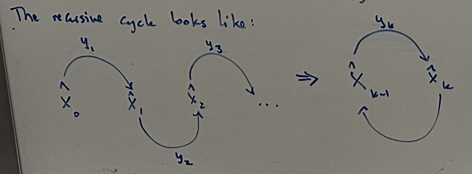
Thus, we want the workflow of the recursive LSE to look like this:

In this diagram, \(\hat{X}_{k-1}\) represents the best-fit model parameters based on the dataset upto the timestep \(k-1\). Once a new datapoint \(y_k\) is introduced, the new model parameters \(\hat{X_{k}}\) are calculated based purely on the previously calculated parameters and the new datapoint.
Recursively Updating the Model Parameters \(\hat{X}_{k}\)
We can start by reordering LSE \((2)\):
\[% \quad \bar{R} = H \bar{X} - \bar{Y} \quad \quad \bar{Y} = H \bar{X} + \bar{R} \quad \tag{1}\]Since we are considering the general case of LSE where datapoints are stochastic (\(\bar{R}\) can also be thought of as random noise), let’s also recall the properties of our (stochastic) datapoints from the Weighted LSE Problem using the Expectation Operator \(E()\) such that:
- \(E(\bar{R}) = 0\) : unbiased, white noise
- mean of the noise (or residual error) across all datapoints is 0
- \(E({r_i}{r_j}^T) = 0\) : no correlation between datapoints
- mean of the covariance between any two datapoints is 0
- this stored in the covariance matrix \(C\)
- \(E({r_i}{r_i}^T) = C_i\) : this is the variance of each measurement. The covariance matrix \(C\) stores these along its diagonal.
Big Picture: The general strategy is to update the model parameters based on the difference between the predicted value (model output) and the actual datapoint. We call this the error or residual \(r_k\) (as we have seen in all of the LSE approaches thus far). We want to therefore update the model parameters by a proportional value \(K_k\) to the magnitude of the residual value. We call \(K_k\) the correction gain.
Thus, the recursive update looks like this:
\[\hat{X}_k = \hat{X}_{k-1} + K_k(R_k)\]where \(R_k = H\hat{X}_{k-1} - Y_k\) :
\[\Rightarrow \boxed{\hat{X}_k = \hat{X}_{k-1} + K_k(H\hat{X}_{k-1} - Y_k)}\]Next, we want to set up this update as an optimization problem in order to minimize the error between our estimate of the best-fit model \(\hat{X}_k\) and the notion of a theoretical best-fit model \(X\).
We will call this error \(\epsilon_k\) such that:
\[\epsilon_k = X - \hat{X}_k\] \[\Rightarrow \epsilon_k = X - (\hat{X}_{k-1} + K_k(H\hat{X}_{k-1} - Y_k))\]We can also note that \(\epsilon_{k-1} = X - \hat{X}_{k-1}\) so:
\[\epsilon_k = \epsilon_{k-1} - K_k(Y_k - H\hat{X}_{k-1})\]Next, we can substitute for \(Y_k\) using \((1)\). In keeping with our current notation, we will re-write \(\bar{X}\) as the more general notation \(X\) to represent the theoretical optimal best-fit parameters. These are the same thing:
\[\epsilon_k = \epsilon_{k-1} - K_k\big[(HX + R_{k}) - H\hat{X}_{k-1}\big]\] \[\Rightarrow \epsilon_{k-1} - K_k\big[(H(X - \hat{X}_{k-1}) + R_{k}\big]\] \[\Rightarrow \epsilon_{k-1} - K_k\big[H\epsilon_{k-1} + R_{k}\big]\] \[\Rightarrow \epsilon_{k-1} - K_{k}H\epsilon_{k-1} - K_{k}R_{k}\]Thus:
\[\epsilon_k = \big(I - K_{k}H\big)\epsilon_{k-1} - K_{k}R_{k}\]If we consider this expression more closely, we can see that:
- the estimation error \(\epsilon_k\) is a function of the previous estimation error and current noise.
- (#TODO: does this make sense?): as long as \(K_{k}H < I\), the new estimation error will be smaller than the previous estimation error.
Recall that we want to minimize the error between the theoretically best-fit parameters \(X\) and the estimated best-fit parameters \(\hat{X}_k\). Since we are recursively updating our estimated best-fit parameters, each update will have some error associated with it.
For further intuition, consider this pattern:
- timestep 1: start with i datapoints and calculate the best-fit line parameters \(\hat{X}_1\). These estimated best-fit parameters might have some estimation error against the overall theoretical best-fit line parameters \(X\) called \(\epsilon_1 = X - \hat{X}_1\)
- timestep 2: when a new datapoint is added, perform the same action. This yields a new estimation error is called \(\epsilon_{2}\)
- … and so on
Similar to our approach with the residuals, we want to square these estimation error components. See the explanation in general LSE for why this is done.
Thus the overall error of the recursive LSE function is the sum of each of these estimation errors. We can call this the overall cost of our error function \(J_k\) such that:
\[J_k = \epsilon_1^{2} + \epsilon_2^{2} + ... + \epsilon_k^{2}\] \[\Rightarrow J_k = (X - \hat{X}_1)^2 + (X - \hat{X}_2)^2 + ... + (X - \hat{X}_k)^2\]If we represent each of our \(\epsilon_i\) components in one vector called \(\epsilon\), we can rewrite our cost function more compactly as:
\[\Rightarrow J_k = \epsilon^{T}\epsilon\]Thus, we can observe that \(J_k\) is expressed through a quadratic function (convex parabola as proven in LSE. This cost is the net error of the recursive LSE function.
Since our control input to drive the estimation error down is \(K_k\) (the gain matrix), we can take the derivative of \(J_k\) with respect to \(K_k\):
\[\frac{\partial J_k}{\partial K_k} = 0 \Rightarrow -2 (I - K_k H) P_{k-1} H^T + 2 K_k C_k\]where \(P_{k}\) can be expressed as:
\[P_k = \epsilon_k \epsilon_k^T\] \[\Rightarrow \big[(I - K_k H_k) \epsilon_{k-1} - K_k R_k\big] \big[ (I - K_k H_k) \epsilon_{k-1} - K_k r_k \big]^T\] \[= (I - K_k H_k) P_{k-1} (I - K_k H_k)^T + K_k R_k K_k^T\]Thus, it works out that our gain matrix \(K_k\) can be expressed as:
\[\boxed{K_k = P_{k-1} H_k^T \left( H_k P_{k-1} H_k^T + C_k \right)^{-1}}\]