Attitude Estimation

High Level Concepts

Our quadrotor flight controller requires a real-time notion of the attitude (3D orientation) of the drone, specifically: pitch, roll and yaw with respect to the inertial frame. We might use an IMU sensor package (accelerometer, gyroscope, magnetometer) to provide this data. However most sensor data is noisy and uncertain or might not even be easily or directly measured.

The point of a state-estimator block then, is to ingest uncertain, noisy sensor data and output the desired attitude signals in real-time, ultimately converging to a high degree notion of the state (in this case attitude).

For now, we will discuss how to estimate roll and pitch, since these can be tracked using purely a gyroscope and accelerometer (packaged in the MPU6050 IMU module).

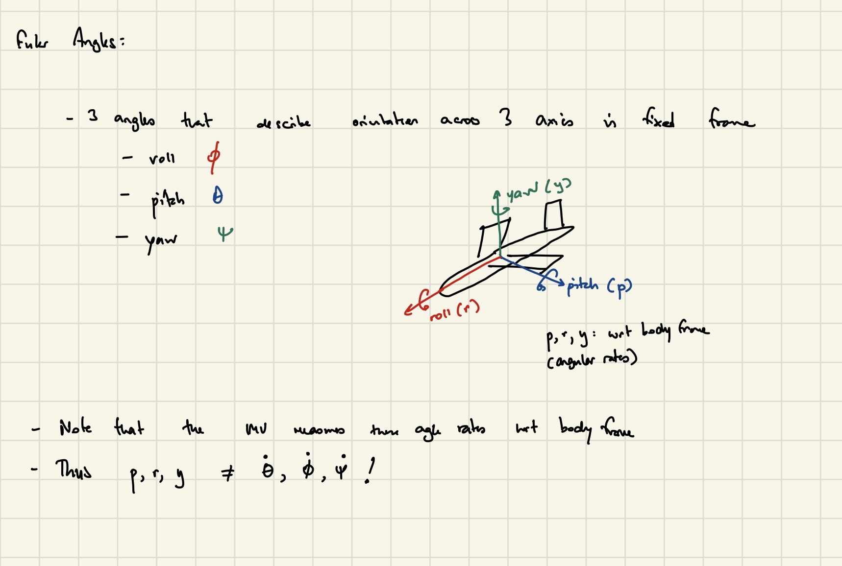
Let’s briefly discuss Euler angles vs. measured angular velocities:

Euler Angles: these are the desired output angles (pitch: \(\theta\), roll: \(\phi\), and yaw: \(\psi\)) that estimate attitude of the drone. They are measured with respect to the inertial frame.

The IMU outputs angular velocities with respect to the body frame (these velocities are called \(p\), \(r\), and \(y\)) in this diagram. Since these are with respect to the body frame, they cannot be considered to be the same as \(\dot{\theta}\), \(\dot{\phi}\) and \(\dot{\psi}\) (these angular rates are with respect to the fixed, inertial frame).

Acclerometer Model

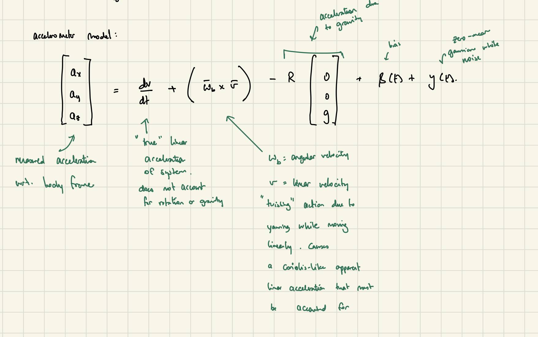
Firstly, let us assume the following coordinate system for the measured accelerometer values. The measured accelerations along the given basis axes of this coordinate system: \(\bar{x}\), \(\bar{y}\) and \(\bar{z}\).

Next, it should be noted that the measured accelerations along these axes are the sum of several components:

• the “true” linear acceleration of the system, not accounting for rotation or gravity
• a coriolis-like acceleration caused by a “twisting” action due to yawing while moving linearly
• acceleration due to gravity, transformed by the orietation of the IMU
• inherent bias that might be built into the accelerometer readings
• zero-mean, unbiased gaussian white noise

How can we derive roll and pitch from these readings?

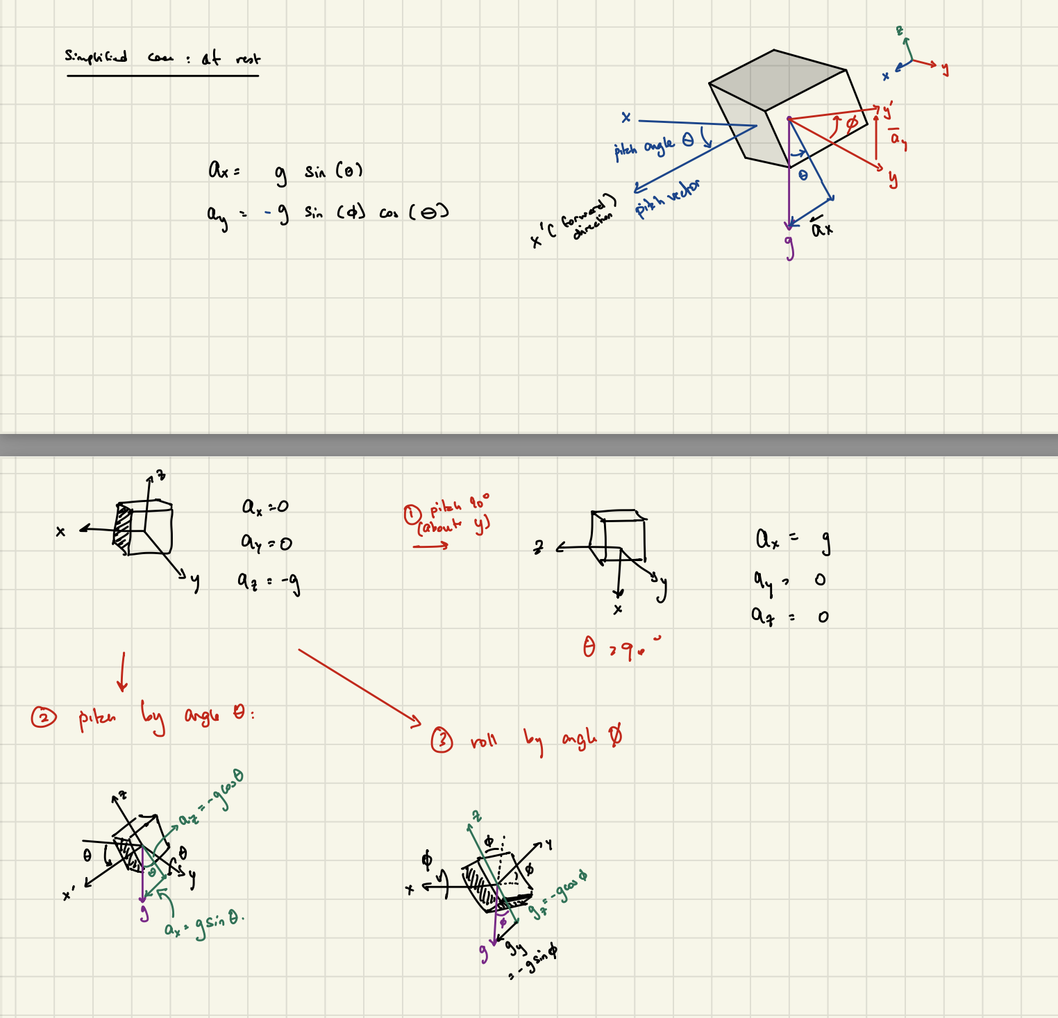
To simplify this model for the purposes of attitude estimation, we will assume that the IMU is at rest.

Therefore, we only consider the component of acceleration due to gravity. The force of gravity is then spread across the three basis vectors of the body frame, proportional to the orientation of the body, manifesting in acceleration readings.

To build an intuition about this relationship, lets consider the effect of pitch and roll individually:

Combining these actions together, we derive the following relationship:

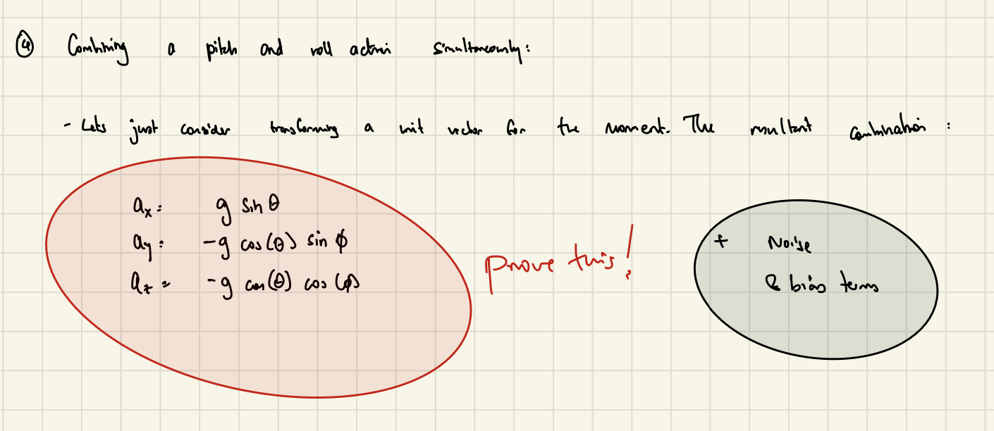
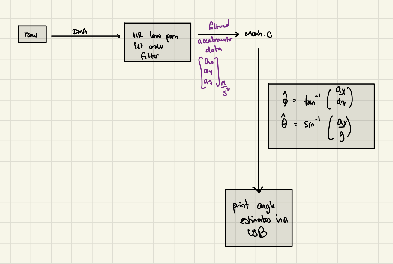
We can then solve for the estimated pitch (\(\hat{\theta}\)) and roll (\(\hat{\phi}\)) with respect to the inertial frame:

\[\frac{a_z}{a_y} = \frac{-g \cos\theta \sin\phi}{-g \cos\theta \cos\phi} = \tan(\phi) \Rightarrow \hat{\phi} = \tan^{-1} \left( \frac{a_z}{a_y} \right)\] \[\frac{a_x}{g} = \frac{g \sin\theta}{g} = \sin\theta \Rightarrow \hat{\theta} = \sin^{-1} \left( \frac{a_x}{g} \right) \\\]

Keep in mind that these estimates are only close to true when the IMU is at rest. While in motion, we need to consider the other acceleration terms, along with the added noise and bias.

Practically, implementing this technique might look like:

Gyroscope Model

Similarly, lets first consider the body coordinate frame of the gyroscope and how it measured angular velocities:

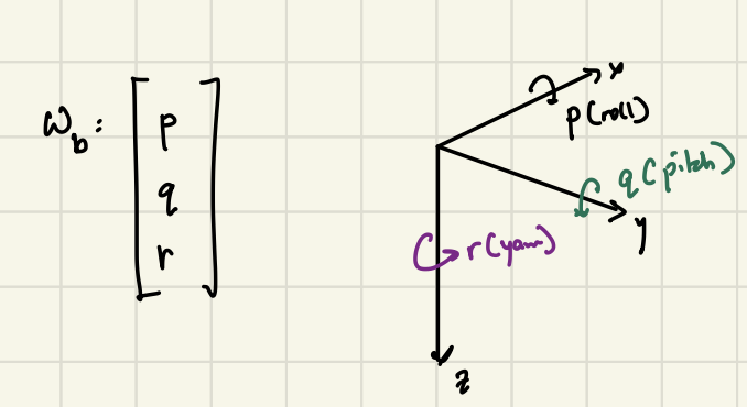
The gyroscope model is relatively simple, with only three components:

• the true angular velocity (in each axis)
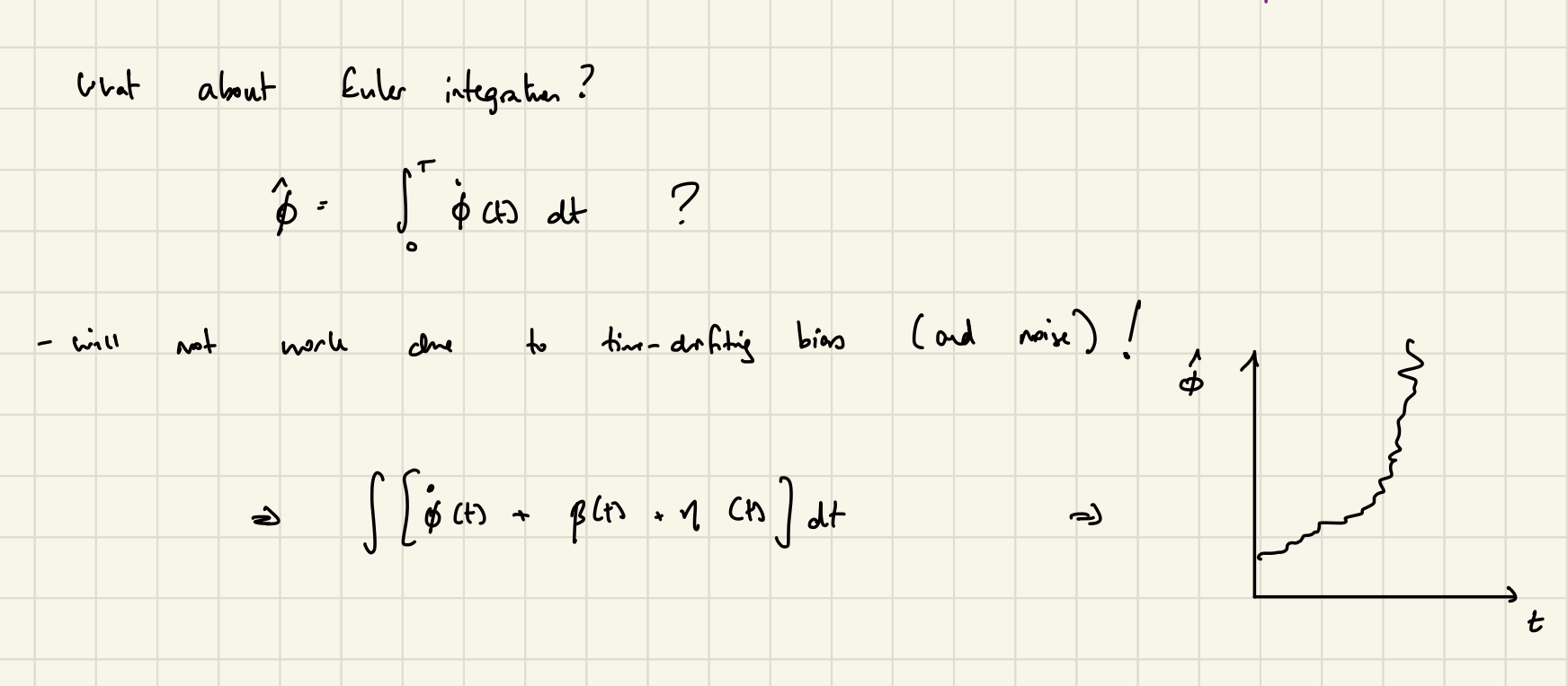
• a time-varying bias that can long term drift in the downstream integration process
• zero-mean, unbiased gaussian white noise

such that:

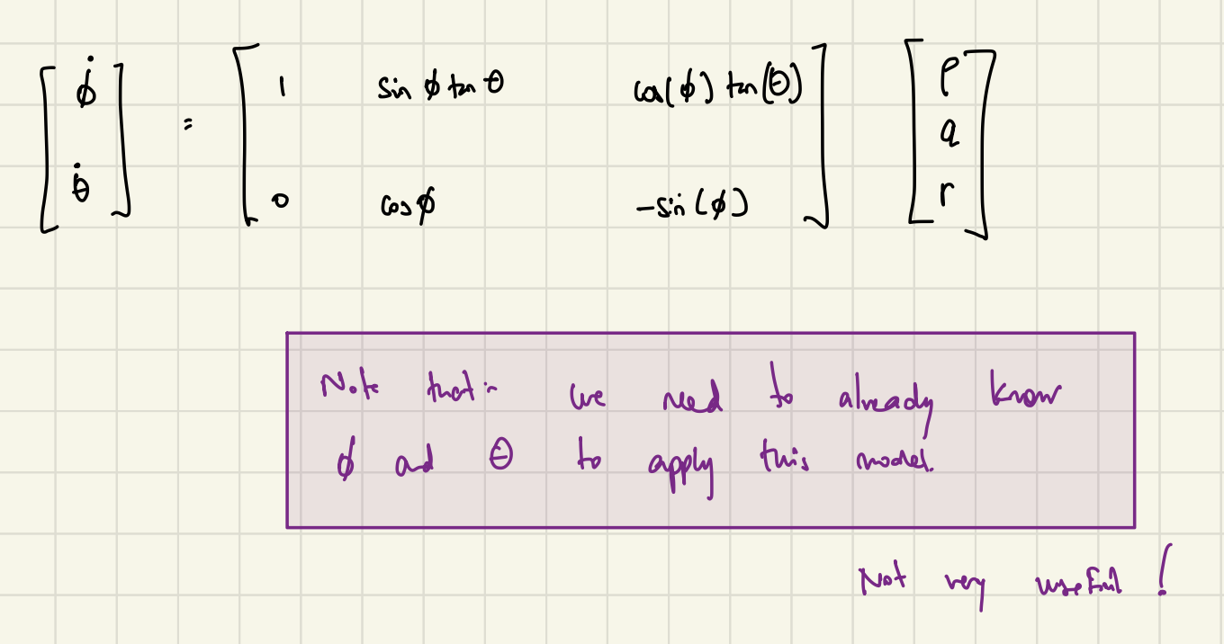
\[\omega{_b} = \omega{_{true}} + \beta{(t)} + \eta{(t)}\]

In order to convert these body-frame angular rates into pitch and roll in the inertial frame, we can refer to this relationship:

Two points of note:

• The output (left-side) shows the pitch and roll angular rates. We will need to apply Euler integration to calculate the actual angles
• This relationship calls for a prior knowledge of \(\theta\) and \(\phi\). Since we don’t know these values, we will need to provide estimated values of these angles from the previous timestep. Any drift or long term error will quickly build up in the subsequent integration step!

Offsetting the Long Term Drift Error

Considering the accuracy of these two modalities:

• Accelerometers give better estimates when they are rest. They tend to generate a lot of white noise when moving.
• Gyroscopes give good readings statically or in-motion for short periods of time. They are prone to drift due to an inherent bias.

When we integrate this inherent bias, we generate a long-term drift error that renders the gyroscope readings too inaccurate to be useful.

If we could find a way to offset this long-term drift error, we could primarily rely on the gyroscope data for real-time attitude estimation.

Solution: since the accelerometer is not particularly accurate in motion but registers white noise (its average reading will be within some reasonable standard deviation of the true value of the attitude), it can limit or “correct” the accumulate drift error per timestep.

Complementary Filters

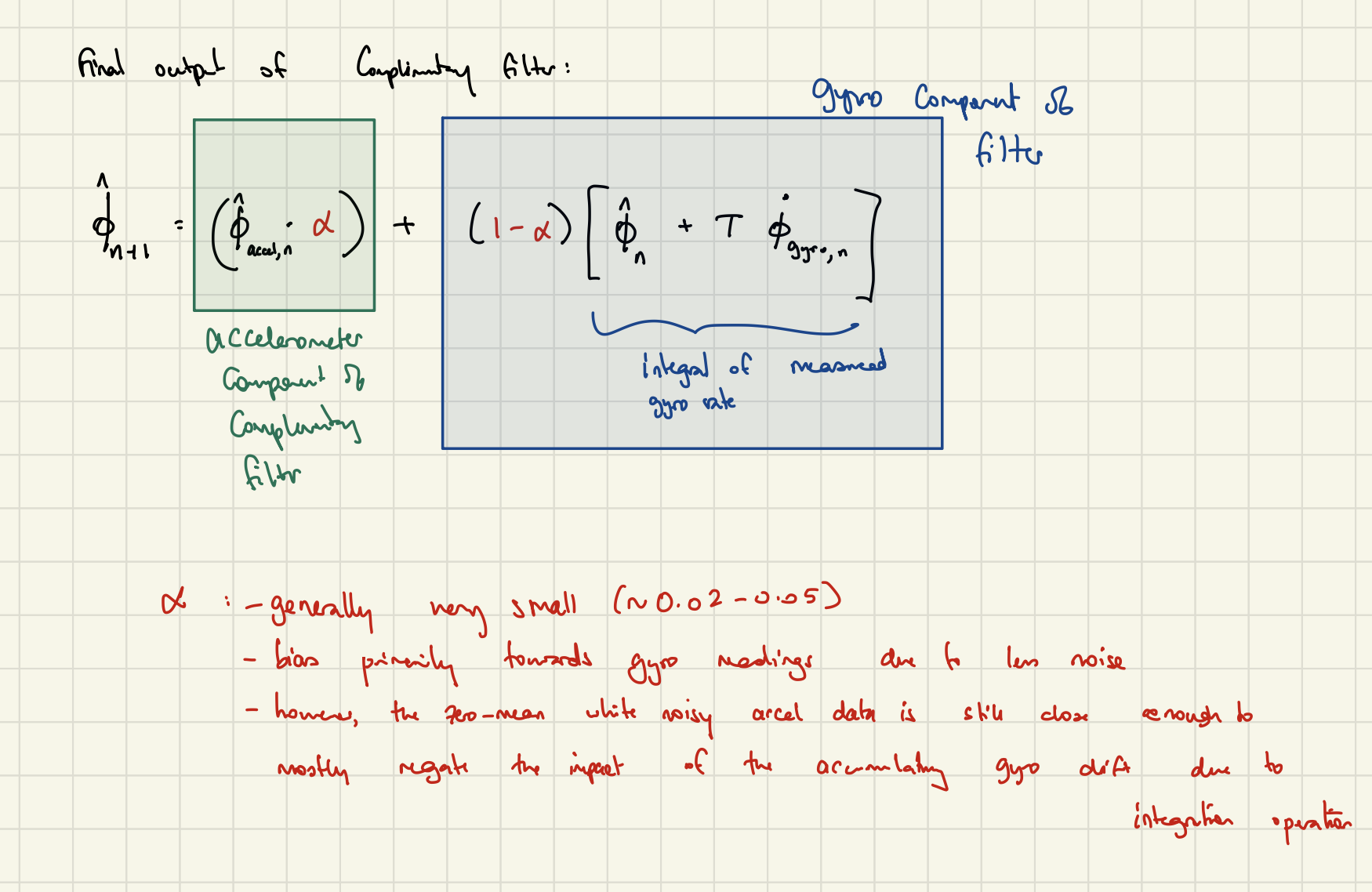
In fact, this is exactly what a complementary filter is. In essence, for each timestemp, our notion of the state is primarily comprised of the gyroscope reading (and integration) with a small component of our notion being influenced by the accelerometer data to negate any build up of long-term drift.

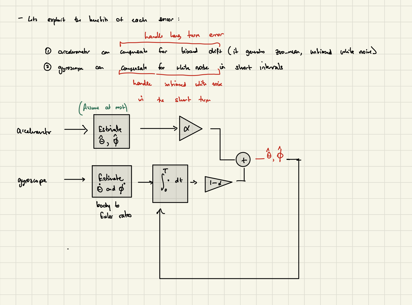
This notion of “small vs primary” components is given by the term \(\alpha\) which signifies “how much confidence we have in our accelerometer readings”. It is usually a very small value, meaning that we trust our short-term gyroscope readings much more.

Extended Kalman Filter

The complementary filter can alternatively be thought of state observer for an LTI state-space model.

Firstly, we can think of the new state \(X_{n+1}\) (attitude) as a function of the current state \(X_n\) and an input \(u\) (in this case, the input would be in the angular velocities read by the gyro):

\[X_{n+1} = AX_n + Bu_n\]

Expanding this out, we have:

\[\begin{bmatrix} \hat{\phi}_{n+1} \\ \hat{\theta}_{n+1} \end{bmatrix} = \begin{bmatrix} 1 & 0 \\ 0 & 1 \end{bmatrix} \begin{bmatrix} \hat{\phi}_{n} \\ \hat{\theta}_{n} \end{bmatrix} + \begin{bmatrix} \tau & 0 \\ 0 & \tau \end{bmatrix} \begin{bmatrix} \dot{\phi} \\ \dot{\theta} \end{bmatrix}\]

We want to subsequently update the gyro-based attitude data by adding the acclerometer correction to handle the long-term drift. This takes on the form of a correction step generated by an “observer”. This allows us to fit the more traditional dynamical systems model by employing a Lunberger observer term to represent the accelerometer correction:

\[X_{n+1} = AX_n + Bu_n + L(X_n - \hat{X_n})\]

where \(X_n\) represents the posterior attitude estimate (of the previous timestamp). Thus, \(Bu_n\) represents influence of the gyro angular velocity readings. On the other hand, \((X_n - \hat{X_n})\) represents the error or “innovation” between the posterior attitude estimate and the current attitude estimate purely from the accelerometer data. Thus the correction step is scaled by the magnitude of the error between the posterior attitude estimate and the current accelerometer estimate.

In the complementary filter, this \(L\) value is a constant, represented as:

\[\begin{bmatrix} \alpha & 0 \\ 0 & \alpha \end{bmatrix}\]

where \(\alpha\) encodes “how much confidence we have in our accelerometer readings”.

In the Kalman filter, lets call this \(K\). It is now called the Kalman Gain and is dynamically evaluated at each timestep. Our equation changes slightly such that the first term is now considered the “prior” (gyro-model estimation) estimate.

The second term is a function of the error between the “true” (accelerometer measurement) state verses the prior estimate, called the innovation term. If these two terms are very different, the correction term should be much larger, causing the posterior (output) estimate to be dramatically different (and corrected).

Given the stochasticity of the two measurement models, our estimate of the state can be represented in a stochastic fashion as well, with a mean and covariance. In this case, the mean is calculated using our LTI + Lunberger equation. The covariance \(P\) can be calculated as the square of the innovation, per the standard definition of the covariance matrix.

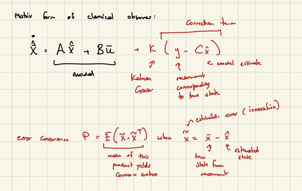
By correcting the prior estimate based on the magnitude of the innovation, the covariance can be expected to be reduced, since it is directly the square of the innovation.

Non-Linear System

We should now note that our system is non-linear, due to all the trigonometric components in our state-space equations. Thus, we can write our state-space system more generally as:

\[\dot{x} = f(x, u) + \xi\] \[ y = h(x, u) + \eta\]

Expanding out the prediction (also called prior and denoted with a superscript \(^-\)) and correction (also called posterior and denoted with a superscript \(^+\)) steps for the estimated mean of the state, we have:

\[\hat{x}_{n+1}^- = \hat{x}_n^+ + T f(\hat{x}_n^+, u)\] \[\hat{x}_{n+1}^+ = \hat{x}_{n+1}^- + K \left(y - h(\hat{x}_{n+1}^-, u) \right)\]

It should be noted that the covariance \(P\) should increase with the prediction step (due to inherent error in the gyroscope reading-integration process), and subsequently decrease once the accelerometer correction is introduced.

Prediction Step:

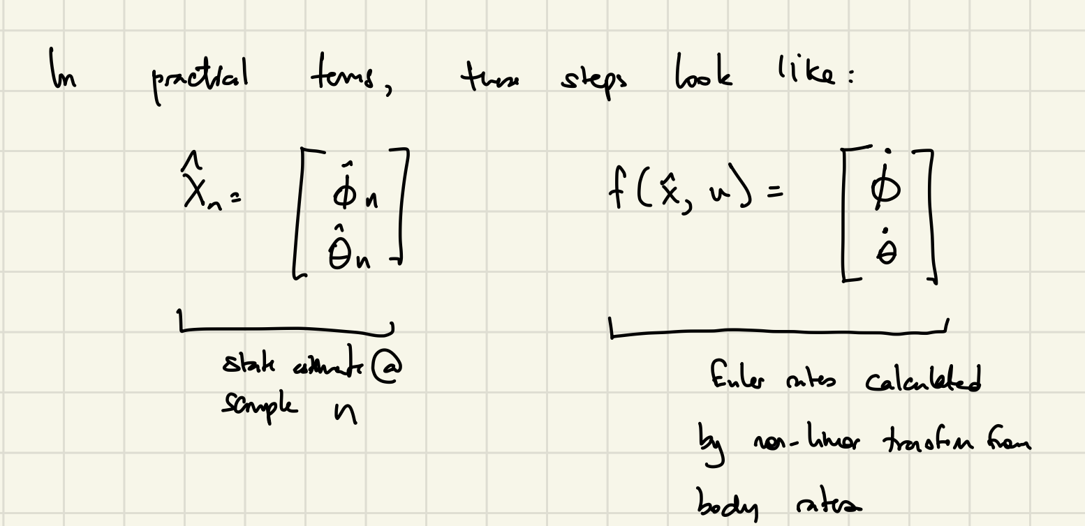
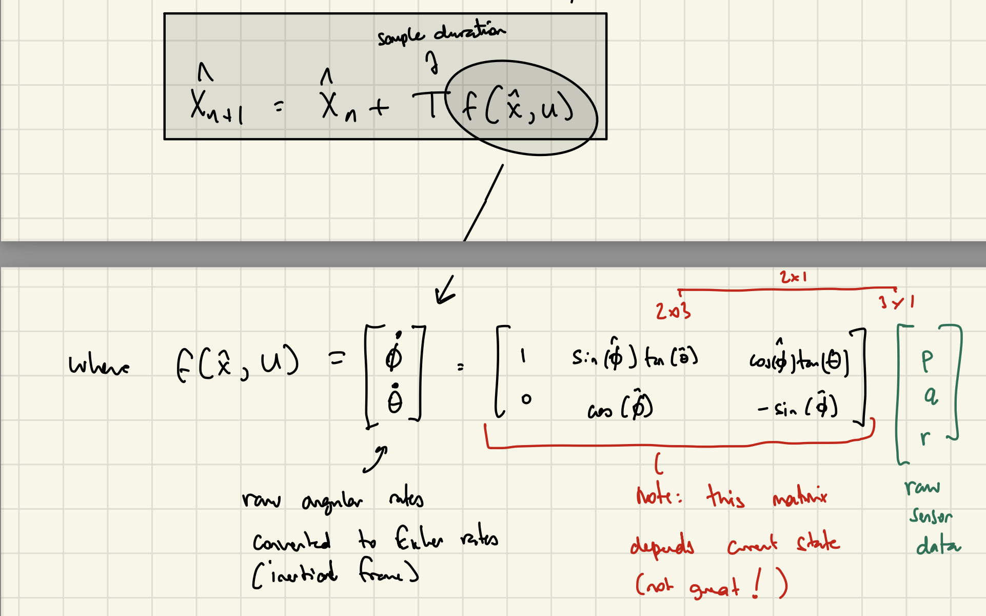
The output attitude rates can then be integrated over the constant timestep T using Euler integration. The final output then is the estimated pitch and roll angle, encoded in \(\hat{X}_{n+1}^-\), also called the estimated prior state.

We also need to update the covariance matrix:

\[P_{n+1}^- = (\nabla{F})P_{n}^{+}(\nabla{F}^T) + JQJ^T\]

Quick Review of Our State-Space System

The general state-space representation of the update step is: \(x_{k+1} = x_k + \Delta t \cdot f(x_k, u_k)\)

where \(f(x_k, u_k)\) represents the mapping of the gyro input (\(u_k\)) from \(p_k\), \(q_k\), \(r_k\) body-frame angular velocities to inertial-frame pitch and roll angular velocities:

\[f(x_k, u_k) = \begin{bmatrix} p_k + q_k \sin(\hat{\phi}) \tan(\hat{\theta}) + r_k \cos(\hat{\phi}) \tan(\hat{\theta}) \\ q_k \cos(\hat{\phi}) - r_k \sin(\hat{\phi}) \end{bmatrix}\]

Thus, our state-space equations can individually be expanded. The estimated prior roll would be: \(\quad \Rightarrow \boxed{\hat{\phi}_{n+1}^{-} = \hat{\phi}_{n}^{+} + \Delta t \cdot \left( p_n + q_n \sin(\hat{\phi_{n}^{+}})\tan(\hat{\theta_{n}^{+}}) + r_n \cos(\hat{\phi_{n}^{+}})\tan(\hat{\theta_{n}^{+}}) \right)}\)

and the estimated prior pitch would be:

$$ \quad \Rightarrow \boxed{\hat{\theta}{n+1}^{-} = \hat{\theta}_n + \Delta t \cdot \left( q_n \cos(\hat{\phi{n}^{+}}) - r_n \sin(\hat{\phi_{n}^{+}}) \right)} $

where \(\nabla{F}\) represents the Jacobian of \(f(x_k, u_k)\), (the mapping of the gyro input to Euler rates). This Jacobian is applied to linearize the non-linear dynamics of the mapping (state transition function). Here, the \(Q\) matrix encodes the process noise covariance (uncertainty in the gyroscope readings).

Since the noise component is assumed to be additive (represented in same state-space by definition so it can be directly added in), \(J\) can be considered to be the \(I\) matrix.

In general, the component \(\nabla{F}P_{n}^{+}\nabla{F}^T\) represents how the uncertainty is re-distributed across the state variables (i.e. no new uncertainty is introduced). The second term \(JQJ^T\) represents the new uncertainty introduced to the system, from the gyroscope measurement uncertainty (in this case).

\[\nabla{F} = \begin{bmatrix} \frac{\partial \dot{\phi}}{\partial \phi} & \frac{\partial \dot{\phi}}{\partial \theta} \\ \frac{\partial \dot{\theta}}{\partial \phi} & \frac{\partial \dot{\theta}}{\partial \theta} \end{bmatrix}\]

Expanding this out, our estimated prior covariance looks like:

\[\quad \Rightarrow \boxed{P_{n+1}^- = (\nabla{F_n})P_{n}^{+}(\nabla{F_n}^T) + Q}\]

where:

\[P_n^+ = \begin{bmatrix} \sigma_{\phi}^2 & \text{Cov}(\phi, \theta) \\ \text{Cov}(\theta, \phi) & \sigma_{\theta}^2 \end{bmatrix}\] \[\nabla{F_n} = \begin{bmatrix} 0 & \sec^2(\theta) (p_n \cos\phi + r_n \sin\phi) \\ -q_n \cos\phi - r_n \sin\phi & 0 \end{bmatrix}\] \[Q_k = \begin{bmatrix} \sigma_p^2 & 0 \\ 0 & \sigma_q^2 \end{bmatrix}\]

Update/Correction Step:

Next, the accelerometer reading \((a_x, a_y, a_z)\) at the current timestep can be used to correct the predicted estimate of the current state.

Thus, the updated state estimate (called the posterior estimate) after correction is:

\[\boxed{\hat{X}_n^+ = \hat{X}_n^- + K(y - h(\hat{X}_n^-, u))}\]

where \(y\) is the measurement, \(h(\hat{X}_n^-, u)\) is the predicted accelerometer measurement and \(K\) is the Kalman gain scaling the effect of the correction step.

The updated convariance is:

\[P^+ = (I - KC)P^-\]

If we expand out the accerometer sensor model \(h(\hat{X}_n^-, u))\), assuming at-rest constraint, we have:

\[h(\hat{X}_k^-, u) = \begin{bmatrix} \hat{a}_{x, k} \\ \hat{a}_{y, k} \\ \hat{a}_{z, k} \end{bmatrix} = g \begin{bmatrix} \sin(\hat{\theta}_k^-) \\ -\cos(\hat{\theta}_k^-) \sin(\hat{\phi}_k^-) \\ -\cos(\hat{\theta}_k^-) \cos(\hat{\phi}_k^-) \end{bmatrix} + \begin{bmatrix} \eta_{x,k} \\ \eta_{y,k} \\ \eta_{z,k} \end{bmatrix}\]

The output (left-hand side) is an estimate of the accelerometer measurement (acceleration in each axis) for the current timestep. This estimate is calculated using the prior estimate of the pitch and roll angles.

Next, due to the at-rest model assumption, the only acceleration to consider is gravity and how it is distributed across the three basis vectors.

Finally, an additive noise component \(\eta\) is appended to the equation, to account of the stochastic element of the measurement.

Why does our correction step look like this?

The correction step is essentially doing this:

1. Determine the “innovation” (error) between the “true state” (given by the actual accelerometer measurement) and predicted accelerometer measurement.
2. The innovation tells us how far our estimated state (using the predicted accelerometer measurement) is from the actual reading.
3. Based on the innovation magnitude, a corrective action updates the estimated state to more closely match the true state.
4. The Kalman Gain encodes how much the measurement should be trusted over the predicted state.

Update Step (continued):

Next, given that the estimated state has an uncertainty, and the sensor measurement is also noisy and therefore has uncertainty, the innovation must also have some uncertainty. We will call this uncertainty \(S_k\) where:

\[S_k = \nabla{h_k}P_k^-\nabla{h_k}^T + R_k\]

where \(\nabla{h_k}\) represents the gradient of the sensor model (used to linearize the non-linear sensor model), and \(R_k\) represents the covariance of the noise component of the measurement (considered additive noise in this case).

Thus, to calculate the Kalman Gain, we can apply the following relationship:

\[\boxed{K_k = P_k^-\nabla{h_x}^TS_k^{-1}}\]

Lastly, the covariance of the posteriori estimate, \(P_k^+\) :

\[\boxed{P_k^+ = (I - K_k\nabla{h_x}_k) P_k^-}\]