Least Squares Estimation (LSE)
High Level Strategy
Suppose you have two points on the x-y plane and you want to find a line that fits the two points. This is easy enough to do using the standard approach of calculating the slope of the line (m = ∆y/∆x) and then using one of the points to calculate the point-slope form of the line: \(y - y_i = b(x - x_i)\) where \((x_i, y_i)\) can be the coordinates of either of the points.
In real-life however, we might have many more than two points, and they will most likely not all fall along the same line. However, we might still want to find a line that models the dataset most accurately. In other words, we want to find the line that best fits the dataset.
How can we do this mathematically?
One way to quantify “accuracy” might be to consider the error or “residual” between each point and the best-fit line. By adding up all the residual components, we can determine the overall error (also called the cost) of the line with respect to the dataset. We can then try to minimize this overall error in some systematic way, proving that we have derived the optimal or best-fit linear model of the dataset.
Let’s add one additional layer of complexity to this approach: instead of simply considering the residual as the raw error between the point and the model at a given x-coordinate, we will consider the square of each residual (hence the name Least Squares Estimate). There are a few advantages to this approach:
- penalize larger errors more: by squaring, we are amplifying the impact of large errors compared to small ones.
- ensure positive error: since we only care about minimizing overall error, we want to consider the magnitude of each residual component.
- differentiable expression of cost: the square of the residuals yields a smooth parabolic function. We will explore why this is ideal.
Suppose we have \(k\) points in our dataset, such that the coordinates of each point can be given by \((x_i, y_i)\). Lets also say that the linear model is given by the expression \(y = bx\). For simplicity, we will start with a model that has a zero y-intercept. Here, the green dots represent the actual points of the dataset with corresponding coordinates. The blue line is our linear model of the data

The above sketch uses red shaded boxes to visualize the square of residuals \((r_1^2, r_2^2, ..., r_k^2)\) where each residual is given by:
\[\begin{aligned} r_1 &= bx_1 - y_1 \\ r_2 &= bx_2 - y_2 \\ &\vdots \\ r_k &= bx_k - y_k \end{aligned}\]So, we can now calculate the overall error of the model as the sum of the squares of these residuals:
\[Error = r_1^2 + r_2^2 + ... + r_k^2\]Looking at this expression more closely by expanding out each residual term, we notice that Error is a function of the b parameter of our linear model. Thus, if we can find the value of b such that Error is minimized, we have derived a specific expression for the best-fit linear model for our dataset.
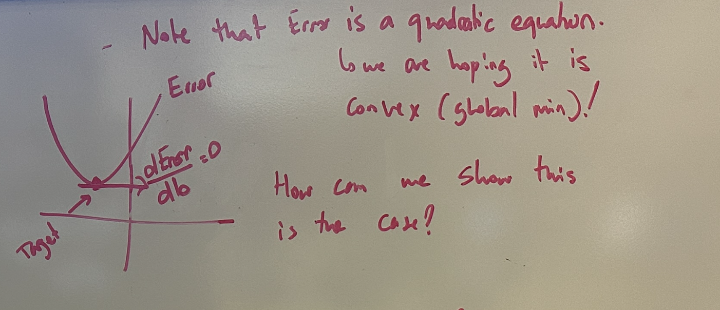
Is this Error function guaranteed to have a global minimum?
We went through the trouble of ensuring our error function is quadratic and therefore has a parabolic profile. In general parabolic function can have a global maximum or a global minimum. For our purposes, we only care about minimizing error: thus, we want our error function to be guaranteed to have a global minimum value. How can we show that this is always the case?

To show this is true, lets start by expanding out the Error function first, and group terms by the b variable:
where the first term: \(\big[ x_1^2 + x_2^2 + \dots + x_k^2 \big]b^2\) is made up of squared values summed together, ensuring that the total will be positive.
Thus, our Error term can be written as a parabolic expression where the 2nd order term has a positive coefficient. In general, this means that the parabola is convex and will have a global minimum. This is ideal because it is relatively easy to compute and there are no edge cases to consider.
Calculating the Corresponding Value of \(b\)
Big Picture: Taking a step back, lets recall what we are doing:
We want to determine the value of \(b\) (the slope) for our linear model that guarantees the model will be the best-fit for our given dataset. We now have an error function (also called a cost function) represented as a convex parabolic function which is dependent on \(b\).
We can therefore calculate the value of \(b\) for which the Error value is minimized. For a parabola, the critical points (minimum or maximum) are located when the derivative of the function is 0. Since the function is convex parabolic, we know there is exactly one global minimum and there are no other critical points (such as saddle points found in higher order functions).
Thus, if we can find the optimal value \(b_{\text{opt}}\) such that the derivative of the Error function \(\frac{d \text{Error}}{db} = 0\), we are done. The linear model \(y = b_{\text{opt}}x\) will be guaranteed to be the best fit for the dataset.
So lets calculate the derivative of the Error function:
\[\frac{d \text{Error}}{db} = 0 \quad \Rightarrow \quad 2b \Big[ x_1^2 + x_2^2 + \dots + x_k^2 \Big] - 2 \Big[ x_1y_1 + x_2y_2 + \dots + x_ky_k \Big] = 0\]Solving for \(b_{\text{opt}}\):
\[b_{\text{opt}} = \frac{\Big[ x_1y_1 + x_2y_2 + \dots + x_ky_k \Big]}{\Big[ x_1^2 + x_2^2 + \dots + x_k^2 \Big]}\]Now our linear model \(y = b_{\text{opt}}x\) is guaranteed to be the best-fit for our dataset.
Least Squares Estimation: The More General Case
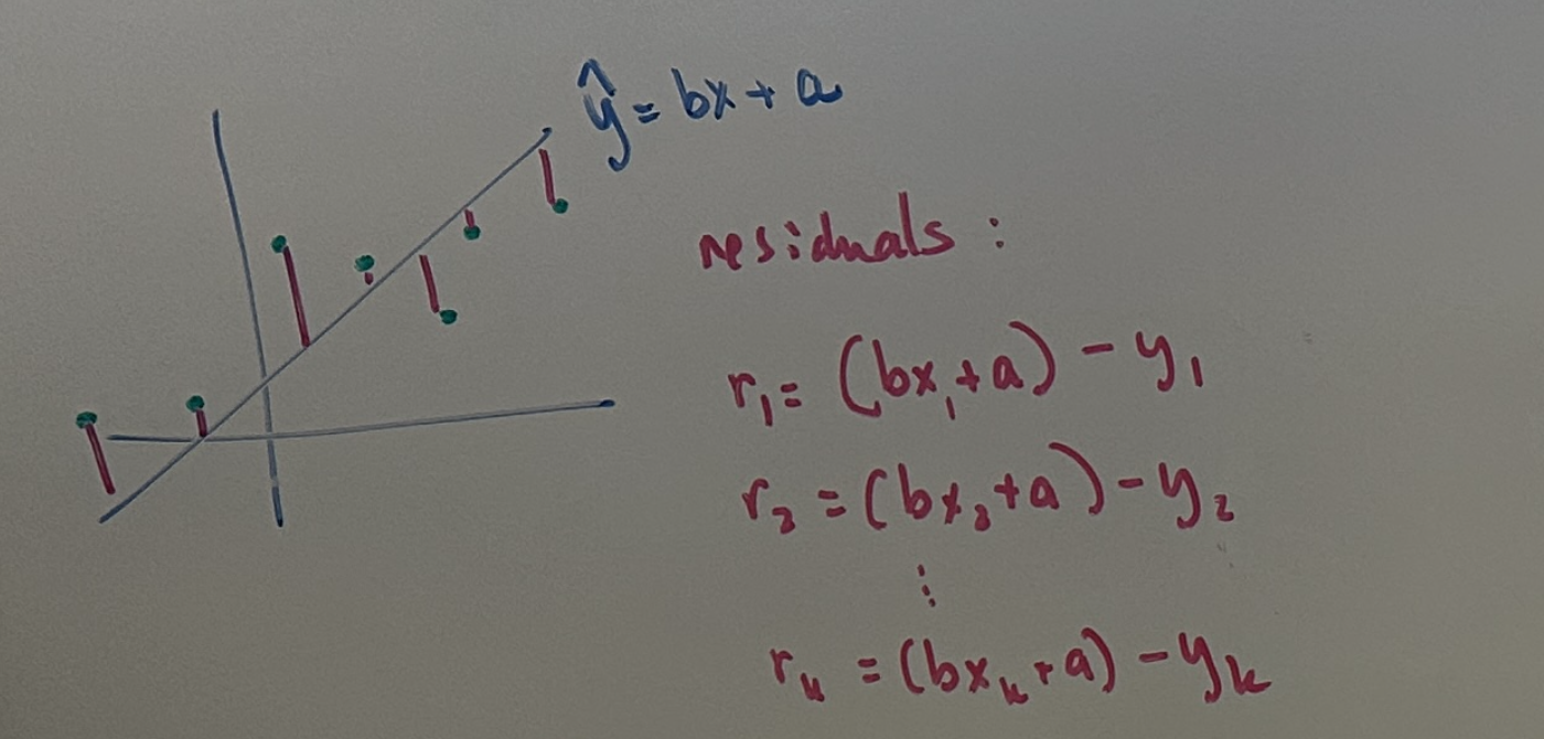
Let’s now consider the more general case of a linear model that is comprised of a slope and a y-intercept. This is more realistic since datasets in the real-world might also introduce a constant bias that can be modeled as an offset in the y-axis.
So our model now looks like:
\[y = bx + a\]where \(a\) represents the y-intercept of the model.
Let’s redraw our dataset, model and residuals:

Once again, we have a system of residual equations (one equation for each of the \(k\) datapoints). This system can be more compactly represented using matrix-vector notation. In addition, matrix-vector notation gives us a variety of useful tools to analyze characteristics of the system as well. For now, let’s start by putting the system in this notation:
\[\begin{bmatrix} r_1 \\ r_2 \\ \vdots \\ r_k \end{bmatrix}_{k \times 1} = \begin{bmatrix} 1 & x_1 \\ 1 & x_2 \\ \vdots & \vdots \\ 1 & x_k \end{bmatrix}_{k \times 2} \begin{bmatrix} a \\ b \end{bmatrix}_{2 \times 1} - \begin{bmatrix} y_1 \\ y_2 \\ \vdots \\ y_k \end{bmatrix}_{k \times 1} \tag{1}\]Here, \(b\) and \(a\) represent the slope and y-intercept parameters respectively of our attempted linear model for this dataset. Ultimately, we are trying to solve for these to generate the best-fit linear model of the dataset.
This notation can be written even more compactly by renaming these matrices and vectors:
\[% \quad \bar{R} = H \bar{X} - \bar{Y} \quad \quad \bar{R} = H \bar{X} - \bar{Y} \quad \tag{2}\]Note: vectors are denoted by bar notation. Thus a vector V is denoted as \(\bar{V}\) in these notes.
Once again, we will need a cost function based on the overall error against which we can optimize our model parameters. The structure of our cost function does not change from our previous LSE case.
\[Error = r_1^2 + r_2^2 + ... + r_k^2\]This error function can also be written compactly in matrix-vector notation:
\[R = \begin{bmatrix} r_1 \\ r_2 \\ \vdots \\ r_k \end{bmatrix}_{k \times 1}, \quad R^T = \begin{bmatrix} r_1 & r_2 & \dots & r_k \end{bmatrix}_{1 \times k}\]so that \(\text{Error} = R^T R \text{ :}\)
\[R^T R = \begin{bmatrix} r_1 & r_2 & \dots & r_k \end{bmatrix}_{1 \times k} \begin{bmatrix} r_1 \\ r_2 \\ \vdots \\ r_k \end{bmatrix}_{k \times 1} = r_1^2 + r_2^2 + \dots + r_k^2\]Now that we have the overall error expression, lets once again find the global minimum of the Error function. However, this time, the error is dependent on two variables: \(b\) (slope) and \(a\) (y-intercept).
In the diagram below, the x-axis and y-axis represent the slope and y-intercept independent variables, and the z-axis (vertical) is the error value. Thus, the error function can be visualized as a 3D shape (paraboloid) with a global mininum:

The intuition to find the global minimum is very similar; we simply need to find the point where the derivative of the error is 0 with respect to the slope and with respect to the y-intercept. Mathematically, each of these conditions can be represented by taking the partial derivative of the Error with respect to each of these variables:
\[\frac{\partial \text{Error}}{\partial a} = 0 \quad \Rightarrow \quad 2r_1 \frac{\partial r_1}{\partial a} + 2r_2 \frac{\partial r_2}{\partial a} + \dots + 2r_k \frac{\partial r_k}{\partial a} = 0\] \[\frac{\partial \text{Error}}{\partial b} = 0 \quad \Rightarrow \quad 2r_1 \frac{\partial r_1}{\partial b} + 2r_2 \frac{\partial r_2}{\partial b} + \dots + 2r_k \frac{\partial r_k}{\partial b} = 0\] \[\Rightarrow \begin{bmatrix} 0 \\ 0 \end{bmatrix} = \begin{bmatrix} \frac{\partial r_1}{\partial a} & \frac{\partial r_2}{\partial a} & \dots & \frac{\partial r_k}{\partial a} \\ \frac{\partial r_1}{\partial b} & \frac{\partial r_2}{\partial b} & \dots & \frac{\partial r_k}{\partial b} \end{bmatrix} \begin{bmatrix} r_1 \\ r_2 \\ \vdots \\ r_k \end{bmatrix} \tag{3}\]Considering the residual error of a given datapoint \(r_i\) more closely: \(r_i = (b x_i + a) - y_i \quad \Rightarrow \quad \frac{\partial r_i}{\partial a} = 1, \quad \frac{\partial r_i}{\partial b} = x_i\)
Thus, we can substitute these expressions for the partial derivative terms for the entire system in \((3)\) as follows:
\[\Rightarrow \begin{bmatrix} 0 \\ 0 \end{bmatrix} = \begin{bmatrix} 1 & 1 & \dots & 1 \\ x_1 & x_2 & \dots & x_k \end{bmatrix} \begin{bmatrix} r_1 \\ r_2 \\ \vdots \\ r_k \end{bmatrix} \tag{4}\]Big Picture: we want to derive the optimal values of the slope \(b\) and y-intercept \(a\) parameters of our linear model. Earlier in this section, we derived a relationship between the residuals and these parameters, as seen in \((2)\). We can take advantage of this.
Note that the multiplier matrix term of the residuals vector in \((4)\) is very similar to the matrix multiplier term \(\bar{H}\) for the model parameters in \((1)\). In fact, they are transposes of each other.
Thus, we can rewrite \((4)\) in matrix-vector form using this notation:
\[\bar{0} = H^T\bar{R} \tag{5}\]Substituting for \(\bar{R}\) from \((2)\), \((5)\) now becomes:
\[\quad \bar{0} = H^T(H \bar{X} - \bar{Y}) \quad \Rightarrow H^TH \bar{X} - H^T\bar{Y}\]The final step is to solve for \(\bar{X}\) (our best-fit linear model parameters):
\[\quad \Rightarrow \boxed{\bar{X} = (H^TH)^{-1}(H^T\bar{Y})}\]This is the general solution for the LSE of the best-fit line for a given dataset.